Pie Of Pie Charts In Excel
Pie Of Pie Charts In Excel - Consider an excel sheet where you have appropriate data to create a chart similar to the below image. Web in this article, i have explained how to make a pie of pie chart in excel. This tutorial demonstrates how to. Here, the secondary pie represents the detailed visualization of the main chart’s slice. Click on the pie chart option within the charts group. On the insert tab, in the charts group, click the pie symbol. Web quickly change a pie chart in your presentation, document, or spreadsheet. Pie charts always use one data series. Web you can compare the relative sizes of other values more easily by breaking out the largest values into a separate pie chart. Select cells > insert > pie of pie. Customizing the appearance of the pie of pie chart and adding data labels and percentages is important for enhancing its visual impact. Pie charts are meant to express a part to whole relationship, where all pieces together represent 100%. Web to make parts of a pie chart stand out without changing the underlying data, you can pull out an individual slice, pull the whole pie apart, or enlarge or stack whole sections by using a pie or bar of pie chart. This is a great way to organize and display data as a percentage of a whole. Web if you want to represent the most significant value from a pie chart, create a pie of pie chart. Click the chart and then click the icons next to the chart to add finishing touches: Web go to the insert tab on the excel ribbon. On the insert tab, in the charts group, click the pie symbol. As the name itself says, a pie of pie chart contains two pie charts. In your spreadsheet, select the data to use for your pie chart. Web creating pie of pie and bar of pie charts. Web go to the insert tab on the excel ribbon. Here, the secondary pie represents the detailed visualization of the main chart’s slice. You can arrange them manually on the sheet. Unlike bar charts and line graphs, you cannot really make a pie chart manually. Here's how to do it. Web if you want to represent the most significant value from a pie chart, create a pie of pie chart. Customizing the pie of pie chart in excel. Adding data labels to pie of pie chart. Web in this article, i have explained how to make a pie of pie chart in excel. Adding data labels to pie of pie chart. Click on the specific pie chart subtype you want to use, and excel will automatically generate a basic pie chart on the worksheet. Or the bar of pie chart: Select data for both pies. How to create a pie chart in excel. As the name itself says, a pie of pie chart contains two pie charts. Bar of pie chart in excel. Click the chart and then click the icons next to the chart to add finishing touches: Change to a pie or bar of pie chart. Pie charts are used to display the contribution of each value (slice) to a total. Inserting a pie of pie chart. How to create a pie chart in excel. Pie charts are meant to express a part to whole relationship, where all pieces together represent 100%. Web go to the insert tab on the excel ribbon. Click the chart and then click the icons next to the chart to add finishing touches: Adding data labels to pie of pie chart. It is actually a double pie chart, which displays the parts of a whole through a main pie, while also providing a way to represent the minor slices through another pie. Web what is pie of pie charts in excel. Click on the pie chart option within the charts group. Then you. Web to create a pie of pie or bar of pie chart, follow these steps: Web in this video, you will learn how to make a pie of pie graph in microsoft excel. I have described the steps including the formatting. Select cells > insert > pie of pie. Web quickly change a pie chart in your presentation, document, or. First, select the range of cells, then click on insert and select pie of pie chart. On the insert tab, in the charts group, click the insert pie or doughnut chart button: Change to a pie or bar of pie chart. Pie charts always use one data series. Click on the pie chart option within the charts group. This tutorial demonstrates how to. Web go to the insert tab on the excel ribbon. On the insert tab, in the charts group, click the insert pie or doughnut chart button: Web creating pie of pie and bar of pie charts. You can arrange them manually on the sheet. Web quickly change a pie chart in your presentation, document, or spreadsheet. Then you can see that the chart was created successfully. Web to make parts of a pie chart stand out without changing the underlying data, you can pull out an individual slice, pull the whole pie apart, or enlarge or stack whole sections by using a pie or. Insert > pie chart > pie of pie. The pie of pie chart: Customizing the appearance of the pie of pie chart and adding data labels and percentages is important for enhancing its visual impact. Here's how to do it. Web what is pie of pie charts in excel. From the insert pie or doughnut chart dropdown list, choose: Inserting a pie of pie chart. How to create a pie chart in excel. In your spreadsheet, select the data to use for your pie chart. Web quickly change a pie chart in your presentation, document, or spreadsheet. Web a pie of pie chart is a pie chart that combines the smallest slices in the chart into one slice and then explodes that slice into a second pie chart. Adding data labels to pie of pie chart. Web in this article, i have explained how to make a pie of pie chart in excel. Click on the pie chart option within the charts group. Or the bar of pie chart: Change to a pie or bar of pie chart.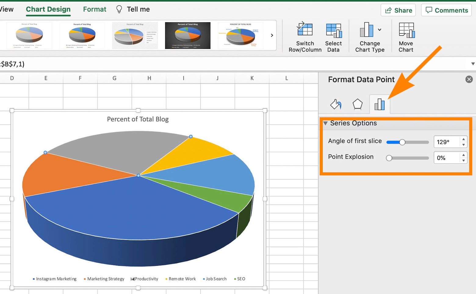
How to Create a Pie Chart in Excel in 60 Seconds or Less
How to Create a Pie Chart in Excel in 60 Seconds or Less

How To Create A Pie Chart In Excel With Multiple Columns Design Talk
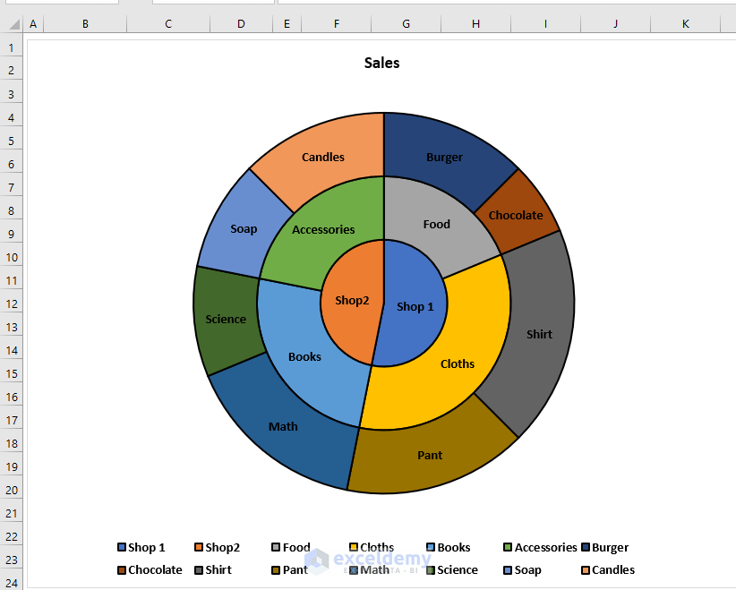
How to Make Pie Chart in Excel with Subcategories (with Easy Steps)
How to create pie chart in excel with data queengai

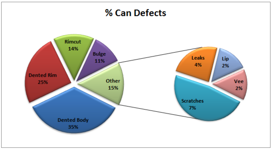
How to Create a Bar of Pie Chart in Excel (With Example)
:max_bytes(150000):strip_icc()/PieOfPie-5bd8ae0ec9e77c00520c8999.jpg)
How to Create Exploding Pie Charts in Excel
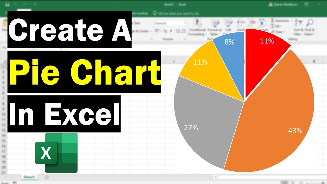
How To Create A Pie Chart In Excel (With Percentages) YouTube

Easily create a dynamic pie of pie chart in Excel

How to Create a Bar of Pie Chart in Excel (With Example)
This Tutorial Demonstrates How To.
In This Example, B3:C12 ).
Click The Chart And Then Click The Icons Next To The Chart To Add Finishing Touches:
This Chart Makes The Pie Chart Less Complicated And Easier To Read.
Related Post: